Dane Eurostatu nt zgonów/urodzeń

Trzeba coś robić w czasie kwarantanny

## https://b-rodrigues.github.io/modern_R/
## https://gist.github.com/imartinezl/2dc230f33604d5fb729fa139535cd0b3
library("eurostat")
library("dplyr")
library("ggplot2")
library("ggpubr")
## 
options(scipen=1000000)
dformat <- "%Y-%m-%d"

eu28 <- c("AT", "BE", "BG", "HR", "CY", "CZ", "DK",
   "EE", "FI", "FR", "DE", "EL", "HU", "IE", 
   "IT", "LT", "LU", "LV", "MT", "NL", "PL", 
   "PT", "RO", "SK", "SI", "ES", "SE")
eu6 <- c("DE", "FR", "IT", "ES", "PL")

### Demo_mor/ Mortality monthly ### ### ###
dm <- get_eurostat(id="demo_mmonth", time_format = "num");
dm$date <- sprintf ("%s-%s-01", dm$time, substr(dm$month, 2, 3))
str(dm)

## There are 12 moths + TOTAL + UNKN
dm_month <- levels(dm$month)
dm_month

## Only new data
dm28  <- dm %>% filter (geo %in% eu28 & as.Date(date) > "1999-12-31")
str(dm28)
levels(dm28$geo) 

## Limit to DE/FR/IT/ES/PL:
dm6  <- dm28 %>% filter (geo %in% eu6)
str(dm6)
levels(dm6$geo) 

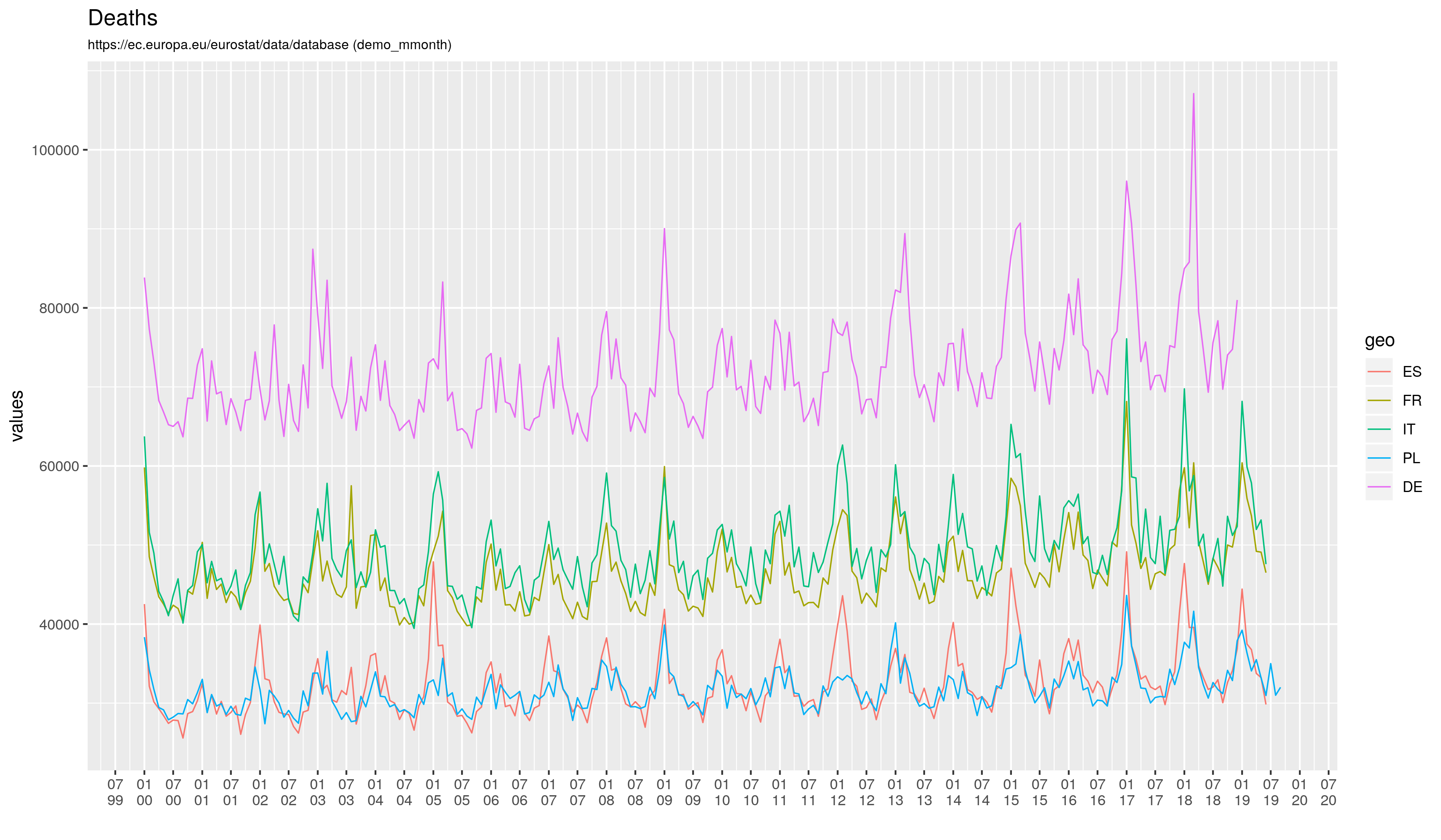
pd1 <- ggplot(dm6, aes(x= as.Date(date, format="%Y-%m-%d"), y=values)) + 
 geom_line(aes(group = geo, color = geo), size=.4) +
 xlab(label="") +
 ##scale_x_date(date_breaks = "3 months", date_labels = "%y%m") +
 scale_x_date(date_breaks = "6 months",
   date_labels = "%m\n%y", position="bottom") +
 theme(plot.subtitle=element_text(size=8, hjust=0, color="black")) +
 ggtitle("Deaths", subtitle="https://ec.europa.eu/eurostat/data/database (demo_mmonth)")

## Newer data
dm6  <- dm6 %>% filter (as.Date(date) > "2009-12-31")

pd2 <- ggplot(dm6, aes(x= as.Date(date, format="%Y-%m-%d"), y=values)) + 
 geom_line(aes(group = geo, color = geo), size=.4) +
 xlab(label="") +
 scale_x_date(date_breaks = "3 months", date_labels = "%m\n%y", position="bottom") +
 theme(plot.subtitle=element_text(size=8, hjust=0, color="black")) +
 ggtitle("Deaths", subtitle="https://ec.europa.eu/eurostat/data/database (demo_mmonth)")

ggsave(plot=pd1, file="mort_eu_L.png", width=12)
ggsave(plot=pd2, file="mort_eu_S.png", width=12)

## Live births (demo_fmonth) ### ### ###

dm <- get_eurostat(id="demo_fmonth", time_format = "num");
dm$date <- sprintf ("%s-%s-01", dm$time, substr(dm$month, 2, 3))
str(dm)

## There are 12 moths + TOTAL + UNKN
dm_month <- levels(dm$month)
dm_month

dm28  <- dm %>% filter (geo %in% eu28 & as.Date(date) > "1999-12-31")
str(dm28)
levels(dm28$geo) 

dm6  <- dm28 %>% filter (geo %in% eu6)
str(dm6)
levels(dm6$geo) 

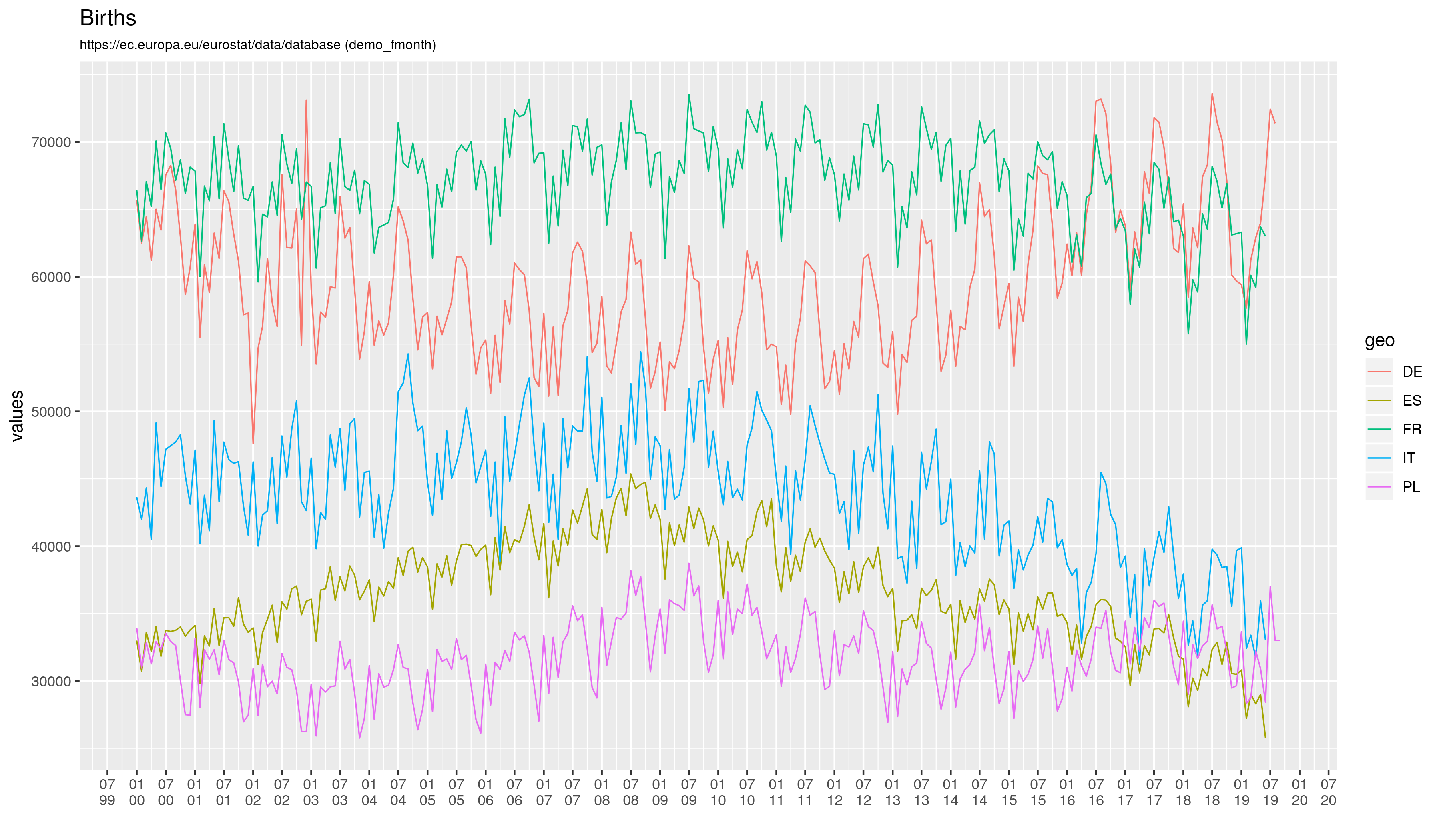
pd1 <- ggplot(dm6, aes(x= as.Date(date, format="%Y-%m-%d"), y=values)) + 
 geom_line(aes(group = geo, color = geo), size=.4) +
 xlab(label="") +
 ##scale_x_date(date_breaks = "3 months", date_labels = "%y%m") +
 scale_x_date(date_breaks = "6 months", date_labels = "%m\n%y", position="bottom") +
 theme(plot.subtitle=element_text(size=8, hjust=0, color="black")) +
 ggtitle("Births", subtitle="https://ec.europa.eu/eurostat/data/database (demo_fmonth)")

##
dm6  <- dm6 %>% filter (as.Date(date) > "2009-12-31")

pd2 <- ggplot(dm6, aes(x= as.Date(date, format="%Y-%m-%d"), y=values)) + 
 geom_line(aes(group = geo, color = geo), size=.4) +
 xlab(label="") +
 scale_x_date(date_breaks = "3 months", date_labels = "%m\n%y", position="bottom") +
 theme(plot.subtitle=element_text(size=8, hjust=0, color="black")) +
 ggtitle("Births", subtitle="https://ec.europa.eu/eurostat/data/database (demo_fmonth)")

ggsave(plot=pd1, file="birt_eu_L.png", width=12)
ggsave(plot=pd2, file="birt_eu_S.png", width=12)

## Population (only) yearly ### ### ##
## Population change - Demographic balance and crude rates at national level (demo_gind)
dp <- get_eurostat(id="demo_gind", time_format = "num");
dp$date <- sprintf ("%s-01-01", dp$time)
str(dp)
dp_indic_dic <-  get_eurostat_dic("indic_de")

dp_indic_dic
dp28  <- dp %>% filter (geo %in% eu28 & time > 1999 & indic_de == "JAN")

str(dp28)
dp6  <- dp28 %>% filter (geo %in% eu6)

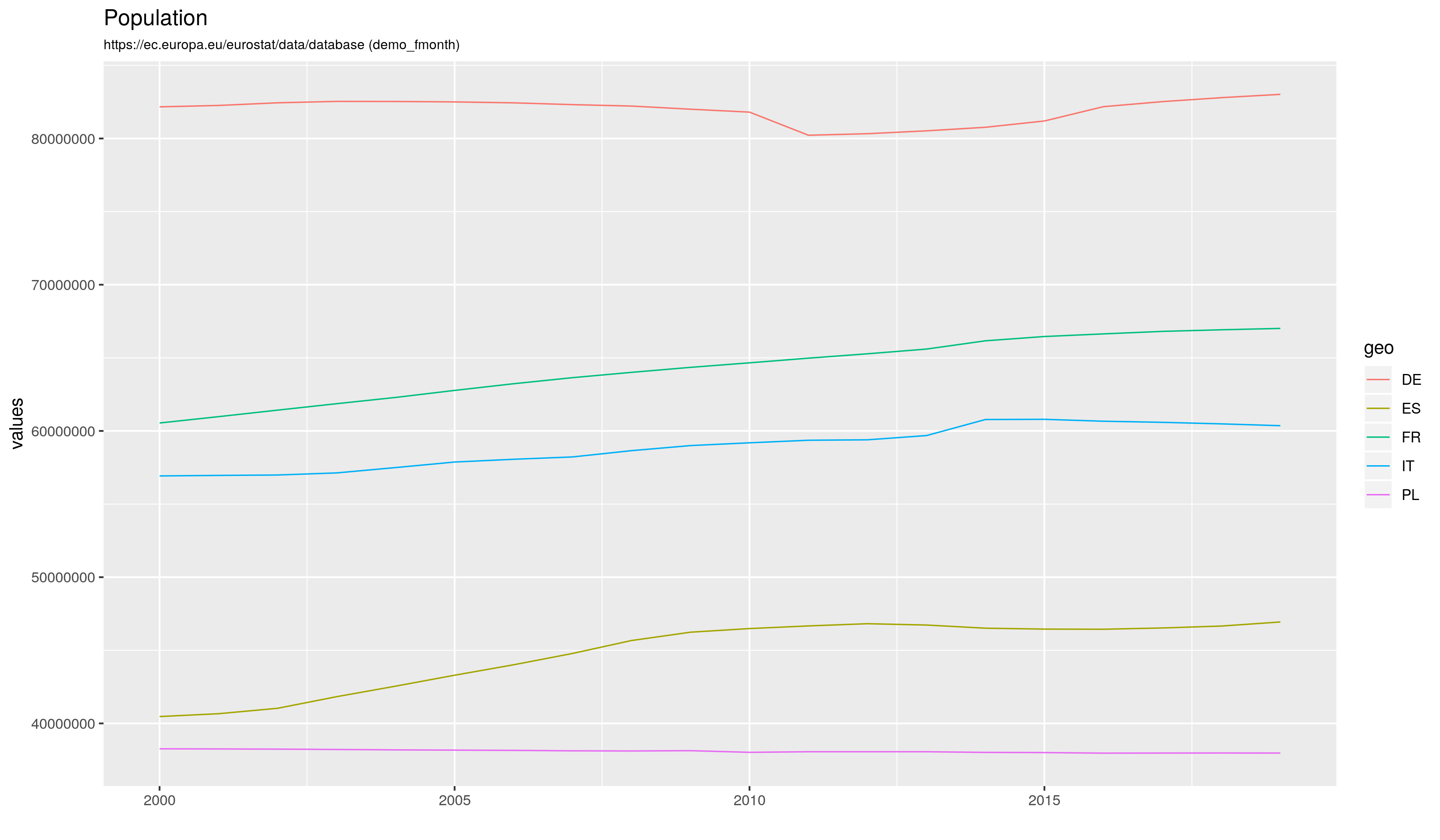
pdp1 <- ggplot(dp6, aes(x= as.Date(date, format="%Y-%m-%d"), y=values)) + 
        geom_line(aes(group = geo, color = geo), size=.4) +
        xlab(label="") +
        ##scale_x_date(date_breaks = "3 months", date_labels = "%y%m") +
        ##scale_x_date(date_breaks = "6 months", date_labels = "%m\n%y", position="bottom") +
        theme(plot.subtitle=element_text(size=8, hjust=0, color="black")) +
        ggtitle("Population", subtitle="https://ec.europa.eu/eurostat/data/database (demo_fmonth)")

ggsave(plot=pdp1, file="pdp1", width=12)