Wględne tempo wzrostu (koronowirusa)

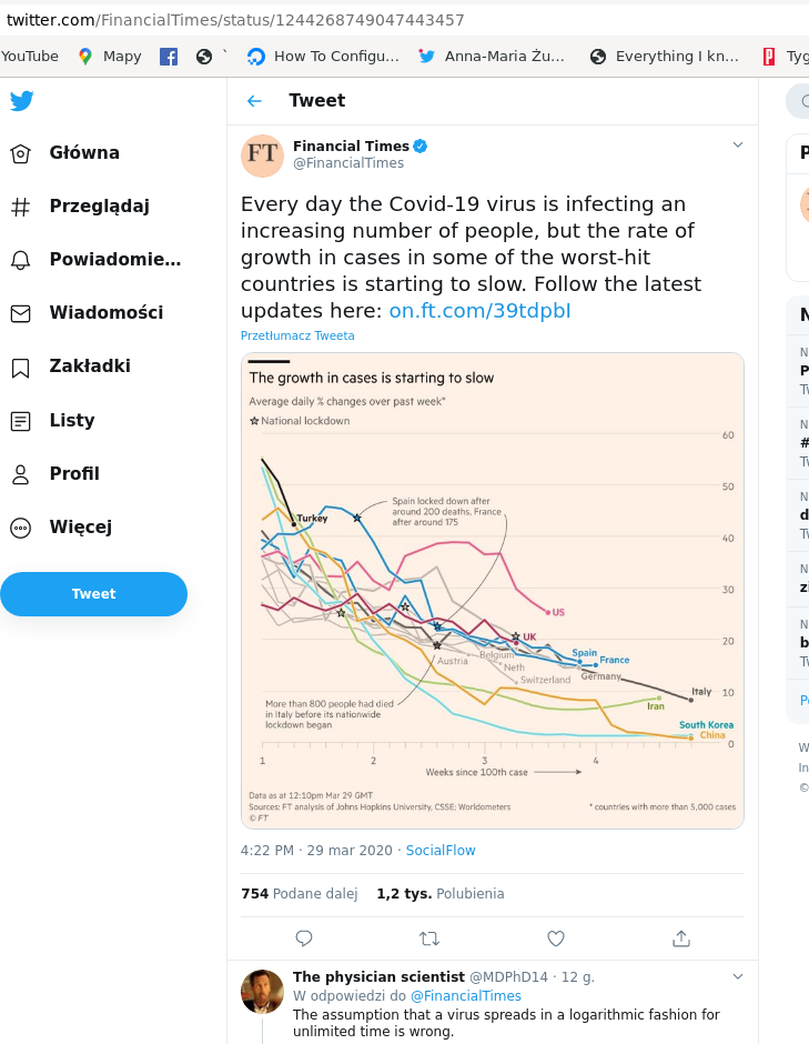
Financial Times zamieścił wykres wględnego tempa wzrostu (rate of growth) czyli procentu liczonego jako liczba-nowych / liczba-ogółem-z-okresu-poprzedniego x 100%. Na wykresie wględnego tempa wzrostu zachorowań na COVID19 wszystkim spada: Every day the Covid-19 virus is infecting an increasing number of people, but the rate of growth in cases in some of the worst-hit countries is starting to slow. Powyższe Czerscy przetłumaczyli jako m.in. trend dotyczy niemal wszystkich krajów rozwiniętych. [he, he... Rozwiniętych pod względem liczby chorych, pewnie chcieli uściślić, ale się nie zmieściło]

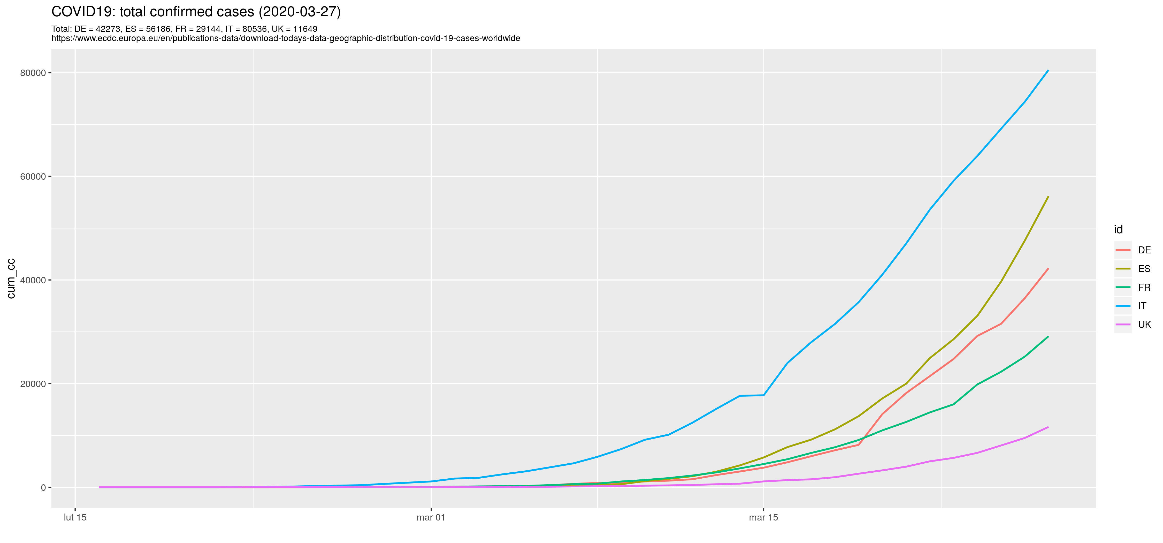
Spróbowałem narysować taki wykres samodzielnie:

library("dplyr")
library("ggplot2")
library("ggpubr")
##
surl <- "https://www.ecdc.europa.eu/en/publications-data/download-todays-data-geographic-distribution-covid-19-cases-worldwide"
today <- Sys.Date()
tt<- format(today, "%d/%m/%Y")

#d <- read.csv("covid19_C.csv", sep = ';',  header=T, na.string="NA", stringsAsFactors=FALSE);
d <- read.csv("covid19_C.csv", sep = ';',  header=T, na.string="NA", 
   colClasses = c('factor', 'factor', 'factor', 'character', 'character', 'numeric', 'numeric'));

d$newc <- as.numeric(d$newc)
d$newd <- as.numeric(d$newd)

Zwykłe read_csv skutkowało tym, że newc/newd nie były liczbami całkowitymi, tylko czynnikami. Z kolei dodanie colClasses kończyło się błędem. W końcu stanęło na tym, że czytam dane w kolumnach newc/newd zadeklarowanych jako napisy a potem konwertuję na liczby. Czy to jest prawidłowa strategia to ja nie wiem...

Kolejny problem: kolumny newc/newd zawierają NA, wykorzystywana później funkcja cumsum z pakietu dplyr, obliczająca szereg kumulowany nie działa poprawnie jeżeli szereg zawiera NA. Zamieniam od razu NA na zero. Alternatywnie można korzystać z funkcji replace_na (pakiet dplyr):

# change NA to 0
d[is.na(d)] = 0

# Alternatywnie replace_na
#d %>% replace_na(list(newc = 0, newd=0)) %>%
#  mutate( cc = cumsum(newc), dd=cumsum(newd))

Ograniczam się tylko do danych dla wybranych krajów, nie starszych niż 16 luty 2020:

d <- d %>% filter(as.Date(date, format="%Y-%m-%d") > "2020-02-15") %>% as.data.frame
str(d)

last.obs <- last(d$date)
c1 <- c('IT', 'DE', 'ES', 'UK', 'FR')
d1 <- d %>% filter (id %in% c1) %>% as.data.frame

str(d1)

Obliczam wartości skumulowane (d zawiera już skumulowane wartości, ale obliczone Perlem tak nawiasem mówiąc):

t1 <- d1 %>% group_by(id) %>%  summarise(cc = sum(newc, na.rm=T), dd=sum(newd, na.rm=T))

t1c <- d %>% group_by(id) %>%  mutate(cum_cc = cumsum(newc), cum_dd = cumsum(newd)) %>% 
  filter (id %in% c1) %>%
  filter(as.Date(date, format="%Y-%m-%d") > "2020-02-15") %>% as.data.frame

  str(t1c)

Wykres wartości skumulowanych:

pc1c <- ggplot(t1c, aes(x= as.Date(date, format="%Y-%m-%d"), y=cum_cc)) + 
  geom_line(aes(group = id, color = id), size=.8) +
  xlab(label="") +
  theme(plot.subtitle=element_text(size=8, hjust=0, color="black")) +
  ggtitle(sprintf("COVID19: total confirmed cases (%s)", last.obs), subtitle=sprintf("%s", surl)) 

ggsave(plot=pc1c, "Covid19_1c.png", width=15)

Kolumny cum_lcc/cum_ldd zawierają wartości z kolumny cum_cc/cum_dd ale opóźnione o jeden okres (funkcja lag):

## 
t1c <- t1c %>% group_by(id) %>% mutate(cum_lcc = lag(cum_cc)) %>% as.data.frame
t1c <- t1c %>% group_by(id) %>% mutate(cum_ldd = lag(cum_dd)) %>% as.data.frame

t1c$gr_cc <- t1c$newc / (t1c$cum_lcc + 0.01) * 100
t1c$gr_dd <- t1c$newd / (t1c$cum_ldd + 0.01) * 100

## Początkowo wartości mogą być ogromne zatem
## zamień na NA jeżeli gr_cc/dd > 90
t1c$gr_cc[ (t1c$gr_cc > 90) ] <- NA
t1c$gr_dd[ (t1c$gr_dd > 90) ] <- NA

Wykres tempa wzrostu:

pc1c_gr <- ggplot(t1c, aes(x= as.Date(date, format="%Y-%m-%d"), y=gr_cc,  colour = id, group=id )) + 
  ##geom_line(aes(group = id, color = id), size=.8) +
  geom_smooth(method = "loess", se=FALSE) +
  xlab(label="") +
  theme(plot.subtitle=element_text(size=8, hjust=0, color="black")) +
  ggtitle(sprintf("COVID19: confirmed cases growth rate (smoothed)"), 
      subtitle=sprintf("%s", surl)) 

ggsave(plot=pc1c_gr, "Covid19_1g.png", width=15)

To samo co wyżej tylko dla PL/CZ/SK/HU:

c2 <- c('PL', 'CZ', 'SK', 'HU')

t2c <- d %>% group_by(id) %>%  mutate(cum_cc = cumsum(newc), cum_dd = cumsum(newd)) %>% 
  filter (id %in% c2) %>%
  filter(as.Date(date, format="%Y-%m-%d") > "2020-02-15") %>% as.data.frame

##str(t2c)
t2c.PL <- t2c %>% filter (id == "PL") %>% as.data.frame
t2c.PL
head(t2c.PL, n=200)

pc2c <- ggplot(t2c, aes(x= as.Date(date, format="%Y-%m-%d"), y=cum_cc)) + 
  geom_line(aes(group = id, color = id), size=.8) +
  xlab(label="") +
  theme(plot.subtitle=element_text(size=8, hjust=0, color="black")) +
  ggtitle(sprintf("COVID19: total confirmed cases (%s)", last.obs), subtitle=sprintf("Total: %s\n%s", lab1c, surl)) 

ggsave(plot=pc2c, "Covid19_2c.png", width=15)

t2c <- t2c %>% group_by(id) %>% mutate(cum_lcc = lag(cum_cc)) %>% as.data.frame
t2c <- t2c %>% group_by(id) %>% mutate(cum_ldd = lag(cum_dd)) %>% as.data.frame

t2c$gr_cc <- t2c$newc / (t2c$cum_lcc + 0.01) * 100
t2c$gr_dd <- t2c$newd / (t2c$cum_ldd + 0.01) * 100

## zamień na NA jeżeli gr_cc/dd > 90
t2c$gr_cc[ (t2c$gr_cc > 90) ] <- NA
t2c$gr_dd[ (t2c$gr_dd > 90) ] <- NA

t2c.PL <- t2c %>% filter (id == "PL") %>% as.data.frame
t2c.PL

pc2c_gr <- ggplot(t2c, aes(x= as.Date(date, format="%Y-%m-%d"), y=gr_cc,  colour = id, group=id )) + 
  ##geom_line(aes(group = id, color = id), size=.8) +
  geom_smooth(method = "loess", se=FALSE) +
  xlab(label="") +
  theme(plot.subtitle=element_text(size=8, hjust=0, color="black")) +
  ggtitle(sprintf("COVID19: confirmed cases growth rate (smoothed)"), 
      subtitle=sprintf("%s", surl)) 

ggsave(plot=pc2c_gr, "Covid19_2g.png", width=15)

Koniec