W mediach podają albo to co było wczoraj, albo razem od początku świata. Zwłaszcza to łącznie od początku ma niewielką wartość, bo są kraje gdzie pandemia wygasa a są gdzie wręcz przeciwnie. Co z tego, że we Włoszech liczba ofiar to 35 tysięcy jak od miesięcy jest to 5--25 osób dziennie czyli tyle co PL, gdzie zmarło do tej pory kilkanaście razy mniej chorych. Podobnie w Chinach, gdzie cała afera się zaczęła, zmarło we wrześniu 15 osób. Media ponadto lubią duże liczby więc zwykle podają zmarłych, a nie zmarłych na 1mln ludności. Nawet w danych ECDC nie ma tego wskaźnika zresztą. Nie ma też wskaźnika zgony/przypadki, który mocno niefachowo i zgrubie pokazywałby skalę zagrożenia (im większa wartość tym więcej zarażonych umiera)
Taka filozofia stoi za skryptem załączonym niżej. Liczy on zmarłych/1mln ludności oraz współczynnik zgony/przypadki dla 14 ostatnich dni. Wartości przedstawia na wykresach: punktowym, histogramie oraz pudełkowym. W podziale na kontynenty i/lub kraje OECD/pozostałe. Ponieważ krajów na świecie jest ponad 200, to nie pokazuje danych dla krajów w których liczba zmarłych jest mniejsza od 100, co eliminuje małe kraje albo takie, w których liczba ofiar COVID19 też jest mała.
Wynik obok. Skrypt poniżej
#!/usr/bin/env Rscript
#
library("ggplot2")
library("dplyr")
#
## Space before/after \n otherwise \n is ignored
url <- "https://www.ecdc.europa.eu/en/publications-data/ \n download-todays-data-geographic-distribution-covid-19-cases-worldwide"
surl <- sprintf ("retrived %s from %s", tt, url)
## population/continent data:
c <- read.csv("ecdc_countries_names.csv", sep = ';', header=T, na.string="NA" )
## COVID data
d <- read.csv("covid19_C.csv", sep = ';', header=T, na.string="NA",
colClasses = c('factor', 'factor', 'factor', 'character', 'character', 'numeric', 'numeric'));
# today <- Sys.Date()
# rather newest date in data set:
today <- as.Date(last(d$date))
# 14 days ago
first.day <- today - 14
tt<- format(today, "%Y-%m-%d")
fd<- format(first.day, "%Y-%m-%d")
# select last row for every country
##t <- d %>% group_by(id) %>% top_n(1, date) %>% as.data.frame
## top_n jest obsolete w nowym dplyr
t <- d %>% group_by(id) %>% slice_tail(n=1) %>% as.data.frame
# cont. select id/totald columns, rename totald to alld
t <- t %>% select(id, totald) %>% rename(alld = totald) %>% as.data.frame
# join t to d:
d <- left_join(d, t, by = "id")
## extra column alld = number of deaths at `today'
##str(d)
# only countries with > 99 deaths:
d <- d %>% filter (alld > 99 ) %>% as.data.frame
## OECD membership data
o <- read.csv("OECD-list.csv", sep = ';', header=T, na.string="NA" )
## Remove rows with NA in ID column (just to be sure)
## d <- d %>% filter(!is.na(id))
d$newc <- as.numeric(d$newc)
d$newd <- as.numeric(d$newd)
cat ("### Cleaning newc/newd: assign NA to negatives...\n")
d$newc[ (d$newc < 0) ] <- NA
d$newd[ (d$newd < 0) ] <- NA
## Filter last 14 days only
d <- d %>% filter(as.Date(date, format="%Y-%m-%d") > fd) %>% as.data.frame
## Last day
last.obs <- last(d$date)
## Format lable firstDay--lastDay (for title):
last14 <- sprintf ("%s--%s", fd, last.obs)
## Sum-up cases and deaths
t <- d %>% group_by(id) %>% summarise( tc = sum(newc, na.rm=TRUE), td = sum(newd, na.rm=TRUE)) %>% as.data.frame
## Add country populations
t <- left_join(t, c, by = "id")
## Add OECD membership
## if membership column is not NA = OECD member
t <- left_join(t, o, by = "id")
t$access[ (t$access > 0) ] <- 'oecd'
t$access[ (is.na(t$access)) ] <- 'non-oecd'
str(t)
## Deaths/Cases ratio %%
t$totr <- t$td/t$tc * 100
## Deaths/1mln
t$tot1m <- t$td/t$popData2019 * 1000000
## PL row
dPL <- t[t$id=="PL",]
##str(dPL)
## Extract ratios for PL
totr.PL <- dPL$totr
totr.PL
tot1m.PL <- dPL$tot1m
## Set scales
pScale <- seq(0,max(t$totr, na.rm=T), by=1)
mScale <- seq(0,max(t$tot1m, na.rm=T), by=10)
## Graphs
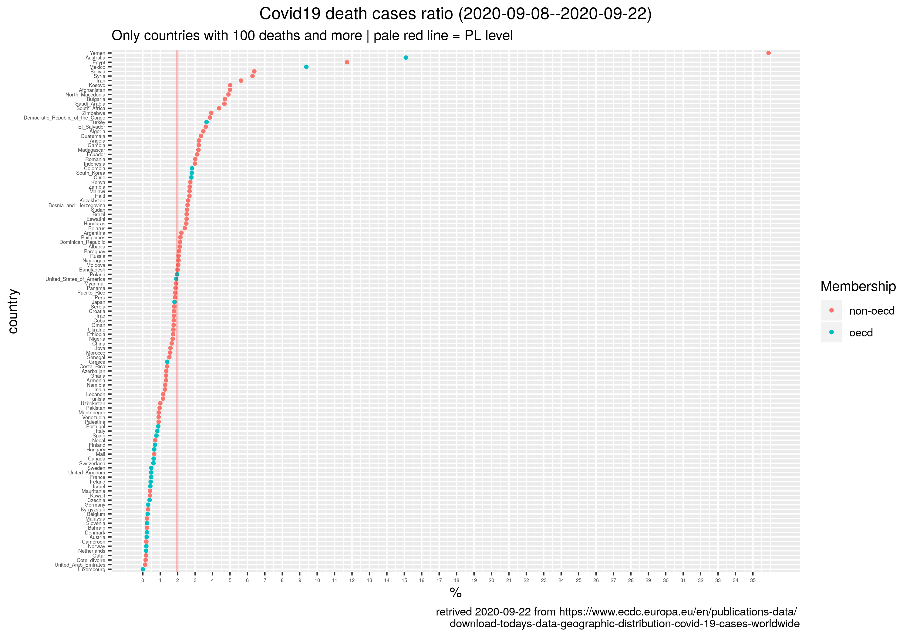
## 1. deaths/cases ratio (dot-plot)
## color=as.factor(access)): draw OECD/nonOECD with separate colors
p1 <- ggplot(t, aes(x = reorder(country, totr) )) +
### One group/one color:
##geom_point(aes(y = totr, color='navyblue'), size=1) +
### Groups with different colors:
geom_point(aes(y = totr, color=as.factor(access)), size=1) +
xlab("country") +
ylab("%") +
ggtitle(sprintf("Covid19 death cases ratio (%s)", last14),
subtitle="Only countries with 100 deaths and more | pale red line = PL level") +
theme(axis.text = element_text(size = 4)) +
theme(plot.title = element_text(hjust = 0.5)) +
##theme(legend.position="none") +
scale_color_discrete(name = "Membership") +
## Indicate PL-level of d/c ratio:
geom_hline(yintercept = totr.PL, color="red", alpha=.25, size=1) +
labs(caption=surl) +
scale_y_continuous(breaks=pScale) +
##coord_flip(ylim = c(0, 15))
coord_flip()
ggsave(plot=p1, file="totr_p14.png", width=10)
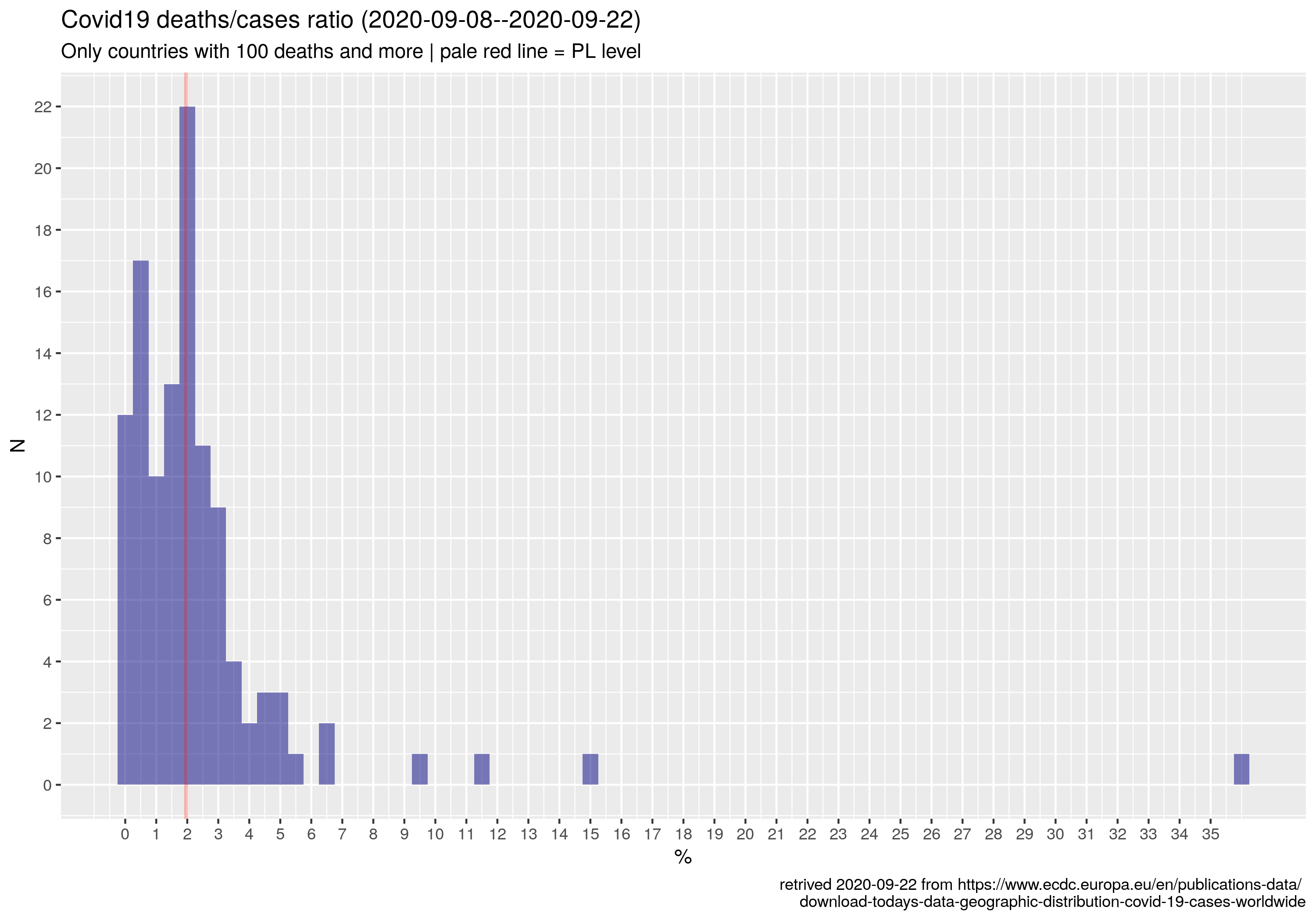
## 2. deaths/cases ratio (histogram)
p2 <- ggplot(t, aes(x = totr) ) +
geom_histogram(binwidth = 0.5, fill='navyblue', alpha=.5) +
###
ylab("N") +
xlab("%") +
ggtitle(sprintf("Covid19 deaths/cases ratio (%s)", last14),
subtitle="Only countries with 100 deaths and more | pale red line = PL level") +
scale_x_continuous(breaks=pScale) +
scale_y_continuous(breaks=seq(0, 40, by=2)) +
geom_vline(xintercept = totr.PL, color="red", alpha=.25, size=1) +
##coord_cartesian(ylim = c(0, 30), xlim=c(0, 8))
labs(caption=surl)
ggsave(plot=p2, file="totr_h14.png", width=10)
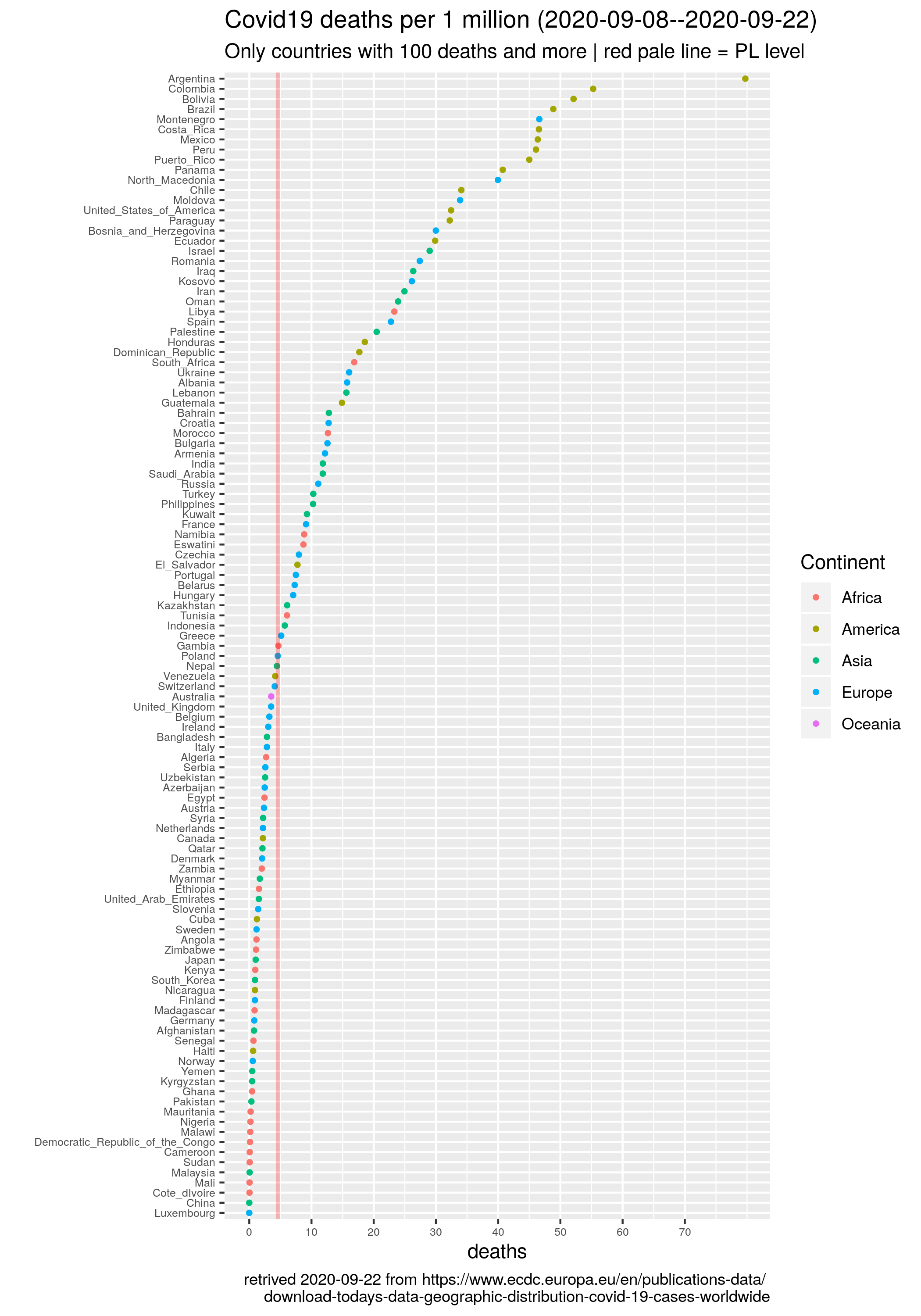
## 3. deaths/1m (dot-plot)
## color=as.factor(continent)): draw continents with separate colors
p3 <- ggplot(t, aes(x = reorder(country, tot1m) )) +
geom_point(aes(y = tot1m, color=as.factor(continent)), size =1 ) +
xlab("") +
ylab("deaths") +
ggtitle(sprintf("Covid19 deaths per 1 million (%s)", last14),
subtitle="Only countries with 100 deaths and more | red pale line = PL level") +
theme(axis.text = element_text(size = 6)) +
geom_hline(yintercept = tot1m.PL, color="red", alpha=.25, size=1) +
labs(caption=surl) +
scale_color_discrete(name = "Continent") +
scale_y_continuous(breaks=mScale) +
coord_flip()
ggsave(plot=p3, file="totr_m14.png", height=10)
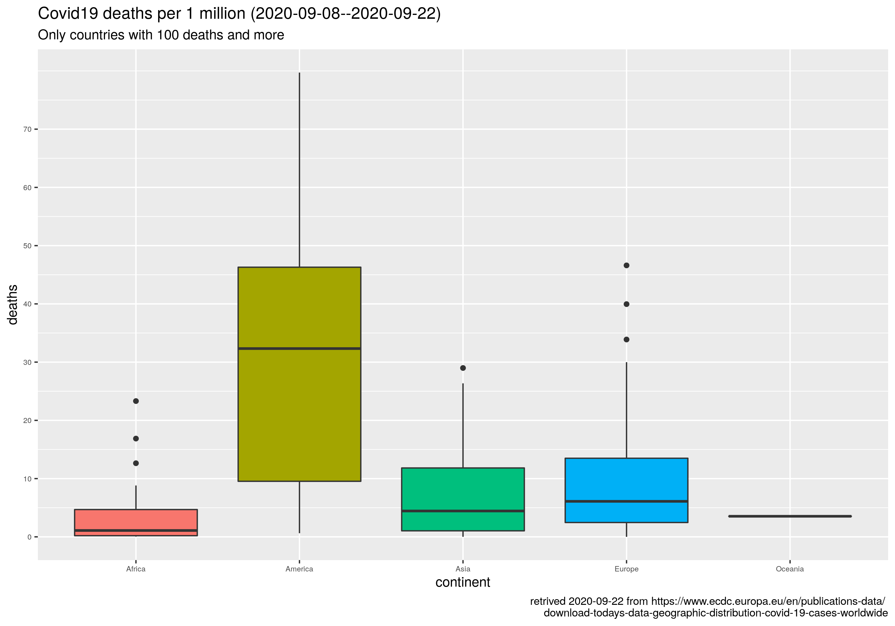
## 3. deaths/1m (box-plots for continents)
p4 <- ggplot(t, aes(x=as.factor(continent), y=tot1m, fill=as.factor(continent))) +
geom_boxplot() +
ylab("deaths") +
xlab("continent") +
ggtitle(sprintf("Covid19 deaths per 1 million (%s)", last14),
subtitle="Only countries with 100 deaths and more") +
labs(caption=surl) +
scale_y_continuous(breaks=mScale) +
theme(axis.text = element_text(size = 6)) +
theme(legend.position="none")
ggsave(plot=p4, file="totr_c14.png", width=10)
## Mean/Median/IQR per continent
ts <- t %>% group_by(as.factor(continent)) %>%
summarise(Mean=mean(tot1m), Median=median(tot1m), Iqr=IQR(tot1m))
ts
Wartość zmarli/przypadki zależy ewidentnie od słynnej liczby testów. Taki Jemen wygląda, że wcale nie testuje więc ma mało przypadków. Z drugiej strony ci co dużo testują mają dużo przypadków, w tym słynne bezobjawowe więc też nie bardzo wiadomo co to oznacza w praktyce. Bo chyba się testuje po coś, a nie żeby testować dla samego testowania. Więc: dużo testów -- na mój niefachowy rozum -- to wczesne wykrycie, a mało to (w teorii przynajmniej) dużo nieujawnionych/nieizolowanych zarażonych, co powinno dawać w konsekwencji coraz większą/lawinowo większą liczbę przypadków, a co za tym idzie zgonów a tak nie jest.
Konkretyzując rysunek: Ameryka na czele liczby zgonów z medianą prawie 30/1mln, Europa poniżej 3,5/1mln a Azja coś koło 1,4/1mln (średnie odpowiednio 26,4/6,00/5,1.)
Przy okazji się okazało, że mam dplyra w wersji 0.8 co jest najnowszą wersją w moim Debianie. No i w tej wersji 0.8 nie ma funkcji slice_head() oraz slice_tail(), która jest mi teraz potrzebna. Z instalowaniem pakietów R w Linuksie to różnie bywa, ale znalazłem na stronie Faster package installs on Linux with Package Manager beta release coś takiego:
RStudio Package Manager 1.0.12 introduces beta support for the binary format of R packages. In this binary format, the repository's packages are already compiled and can be `installed' much faster -- `installing' the package amounts to just downloading the binary!
In a configured environment, users can access these packages using `install.packages' without any changes to their workflow. For example, if the user is using R 3.5 on Ubuntu 16 (Xenial):
> install.packages("dplyr", repos = "https://demo.rstudiopm.com/cran/__linux__/xenial/latest")
Zadziałało, ale (bo jest zawsze jakieś ale) powtórzenie powyższego na raspberry pi nie zadziała. Wszystko się instaluje tyle że architektury się nie zgadzają. Więc i tak musiałem wykonać
> install.packages("dplyr")
## sprawdzenie wersji pakietów
> sessionInfo()
Instalacja trwała 4 minuty i zakończyła się sukcesem.
Brak komentarzy:
Prześlij komentarz